GAN

Deep-learning · 12 Jun 2019

Source code: Everyone can run the code in Colab envrionment with the GPU.

Generative Adversarial Network (GAN) is a generative framework besides variationall autoencoders which introduces the minmax game theory into unsupervised learning. I have implementated the original GAN propsed by Ian Goodfellow and another improved version for the MNIST digits dataset using the beta version Tensorflow 2.0 library. The encounted problems are documented here. Meanwhile, the possible solutions for notorious GAN training problems are analyzed. It is helpful to get familiar with the practical GAN problems and understand the effect of different network properties. This is also an example to show the Tensorflow 2.0 style.

Vanilla GAN

Vanilla GAN is the original and simplest form proposed in 2014. The main concept is to simultaneously tain two neural networks: one is Generator (G) which learns the real data distribution, the other is Discriminator (D) which determines the liklihood of the sample from the data distribution. Therefore, this is a minmax two-player game where generator represents the fake painters and the discriminator is like the judges. These two agents have the same value function that one seeks to maximize and another to minimize. Eventually, the game ends at the saddle point, which is the minimum for one agent and the maximum for another. At this saddle point, the hession of the value function is zero, which indicates the learning process stops.

The simplest value function is:

\[\min_G \max_D V(G, D) = \mathbb{E}_{x ~ p_{data}}[log D(x)] + \mathbb{E}_{z ~ p_z}[log (1-D(G(z)))]\]

where $p_{data}$ is the true data distribution, $p_z$ is a prior of the input noise.

Regarding the discriminator, it learns to correctly distinguish between the fake samples from the generator and the real samples, as we seperate its value function:

\[\max_D V = \mathbb{E}_{x ~ p_{data}}[log D(x)] + \mathbb{E}_{z ~ p_z}[log (1-D(G(z)))]\]

In the extreme cases, it scores the fake samples as 0, and the true samples as 1.

Regarding the generator, it learns to cheat the discriminator by capturing the true data distribution. At the extreme cases, $D(G(z)) = 1$. And the value function ends up with minus infinity.

\[\min_G V = \mathbb{E}_{z ~ p_z}[log (1-D(G(z)))]\]

Since the gradient of the above value function can be vanished at the very beginning of the training due to the poor performance of generator, the author proposes to use:

\[\max_G V = \mathbb{E}_{z ~ p_z}[log D(G(z))]\]

The code of this value function is:

def loss_discriminator(sample_data, sample_generator):
  pred_data_logits = discriminator(sample_data)
  pred_gen_logits = discriminator(sample_generator)
  
#   loss_dis = -tf.reduce_mean(tf.math.log(pred_data)+tf.math.log(1.0-pred_generator))
  loss_data = tf.reduce_mean(tf.nn.sigmoid_cross_entropy_with_logits(labels=tf.ones_like(pred_data_logits), logits=pred_data_logits))
  loss_gen_sample = tf.reduce_mean(tf.nn.sigmoid_cross_entropy_with_logits(labels=tf.zeros_like(pred_gen_logits), logits=pred_gen_logits))
  loss_dis = loss_data+loss_gen_sample
  
  
  return loss_dis

def loss_generator(sample):
#   loss = -tf.reduce_mean(tf.math.log(discriminator(sample)))
  pred_logits = discriminator(sample)
  loss = tf.reduce_mean(tf.nn.sigmoid_cross_entropy_with_logits(labels=tf.ones_like(pred_logits), logits=pred_logits))
  
  return loss

Notice that I use the internal existing function sigmoid_cross_entropy_with_logits to avoid numerical errors.

In this vanilla GAN, I use a simple feedforward networks for the MNIST dataset, which is shown as below:

In Tensorflow 2.0, the model is implemented as:

class Generator(Model):
  def __init__(self):
    super(Generator, self).__init__()
    self.d1 = tf.keras.layers.Dense(128, activation='relu')
    self.d2 = tf.keras.layers.Dense(128, activation='relu')
    self.d3 = tf.keras.layers.BatchNormalization()
    self.d4 = tf.keras.layers.Dense(28*28, activation='tanh')

  def call(self, x):
    x = self.d1(x)
    x = self.d2(x)
    x = self.d3(x)
    return self.d4(x)

class Discriminator(Model):
  def __init__(self):
    super(Discriminator, self).__init__()
    self.d1 = tf.keras.layers.Dense(256, activation='relu')
    self.d2 = tf.keras.layers.Dense(256, activation='relu')
    self.d3 = tf.keras.layers.Dropout(0.2)
    
    self.d4 = tf.keras.layers.Dense(1, activation=None)

  def call(self, x):
    x = self.d1(x)
    x = self.d2(x)
    x = self.d3(x)
    x = self.d4(x)
    return tf.keras.activations.sigmoid(x), x

A very useful feature of Tensorflow 2.0 is the implicit graph building triggered by the python decorator tf.function. It is much easier and clear to do the training process:

@tf.function
def train_step():
  ind = np.random.choice(x_train.shape[0], size=BATCH_SIZE)
  sample = x_train[ind,:]
  
  sample_gen = generator(norm_sample(BATCH_SIZE, INPUT_FEATURE), True)

  loss_dis, grad_dis = f_grad_dis(discriminator, sample, sample_gen)

  optimizer_dis.apply_gradients(zip(grad_dis, discriminator.trainable_variables))

  ls_dis.update_state(loss_dis)
   
  with tf.GradientTape()as g_gen:
    sample_gen = generator(norm_sample(BATCH_SIZE, INPUT_FEATURE), True)
    loss_gen = loss_gen(sample_gen)
  
  grad_gen = g_gen.gradient(loss_gen, generator.trainable_variables)
  optimizer_gen.apply_gradients(zip(grad_gen, generator.trainable_variables))
  
  ls_gen.update_state(loss_gen)
  
  
  return loss_dis, loss_gen

Training

The training configuration parameters are summarized as:

Learning rate	1e-3
Beta1 (Adam optimizer)	0.5

Generator

Learning rate	1e-4
Beta1 (Adam optimizer)	0.5

Discriminator

Batch size	128
Noise dimention	100
Noise type	Gaussian
Epoch	80

Training

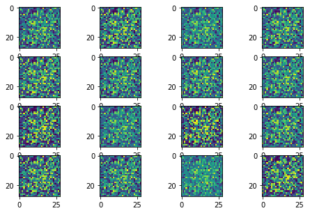
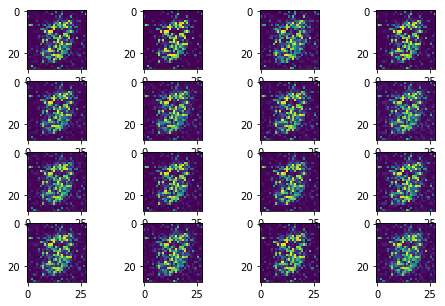
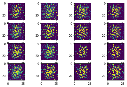
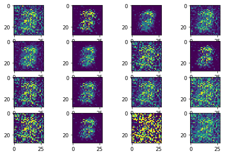
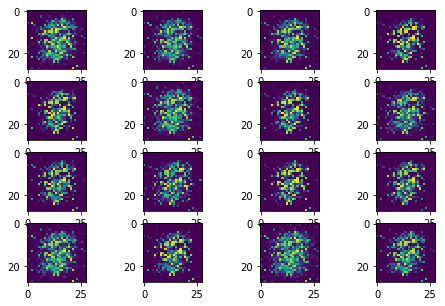
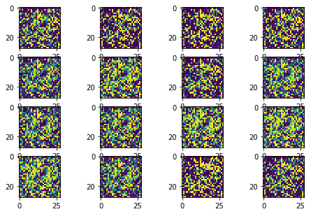
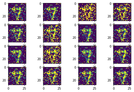
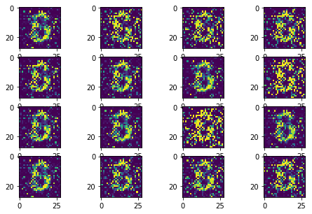
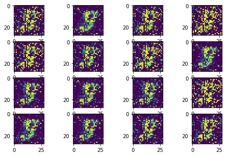
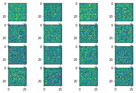
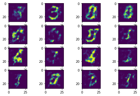
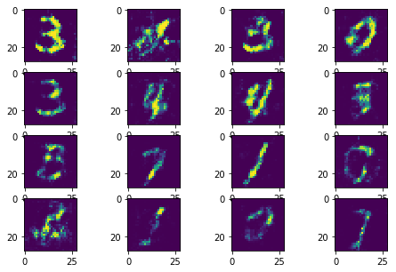
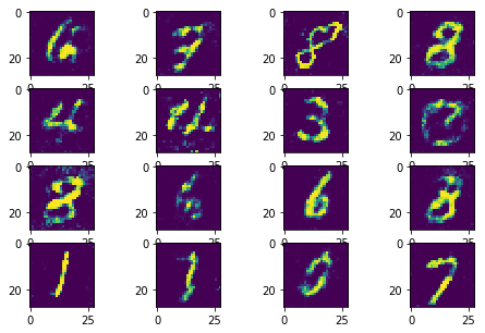
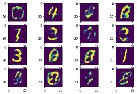
The following sequence of images show the learning process of the generator:

And the loss curves roughly look like:

Problems

The training process shows two serious problems about the GAN training.

Mode collapse

Instead of learning the rich data distributions over all possible modes, GAN collapes to a single mode. Therefore, it generates a similar number however the input noise changes.

Training stability

The training process could repeat the learning process from total noise to some meaningful distributions, as it can be identified from the loss curve. Therefore, the convergence of the learning can not be guaranteed.

Wasserstein Loss

To solve these problems, Ishaan et al. proposed Wasserstein GAN with gradient penalty. The WGAN value function is:

\[\min_G \max_{D \in \mathcal{D}} \mathbb{E}_{x ~ p_{data}} [D(x)] - \mathbb{E}_{x ~ G(z)} [D(x)]\]

where $\mathcal{D}$ is the set of 1-Lipschitz functions. This WGAN value function has better gradient flows compared with the original GAN. The gradient penalty method is proposed to fulfill the Lipschitz constraints. It is defined as:

\[R = \lambda \mathbb{E}_{\hat{x} ~ p_{\hat{x}}} [(||\nabla_{\hat{x}} D(\hat{x})||_2-1)^2]\]

where $p_{\hat{x}}$ is the uniform interpolation between the real data samples and the generated data samples.

This gradient penalty is added to the discriminator loss according to the definition of 1-Lipschtiz function:

A differentiable function is 1-Lipschtiz if and only if it has gradients with norm at most 1 everywhere.

def loss_dis_wass(sample_data, sample_generator, lam):
  pred_data_logits = discriminator(sample_data)
  pred_gen_logits = discriminator(sample_generator)
  
  loss_dis = tf.reduce_mean(pred_gen_logits) - tf.reduce_mean(pred_data_logits)
  
  # gradient penalty
  epsilon = tf.random.uniform(shape=(BATCH_SIZE,1,1,1), minval=0, maxval=1.0)
  diff = sample_generator - sample_data
  interpolation = sample_data + epsilon*diff
  g = tf.gradients(discriminator(interpolation), [interpolation])
  EPS = 1e-10
  slopes = tf.sqrt(tf.reduce_sum(tf.square(g), axis=[1,2,3])+EPS)
  loss_dis += lam*tf.reduce_mean((slopes - 1.0)**2)
  return loss_dis

def loss_gen_wass(sample):
  pred_logits = discriminator(sample)
  loss = -tf.reduce_mean(pred_logits)
  return loss

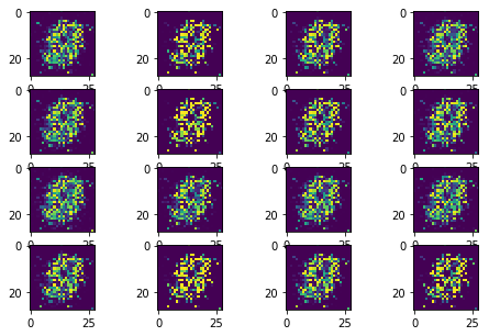
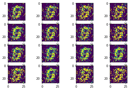
Improved GAN

Besides the change of the loss function, I also update the model architect to efficiently capture the image features by convolution layers.

Note: Some dropouts and batch normalization layers are not shown in the figure.

Training

Learning rate	1e-3
Beta1 (Adam optimizer)	0.5

Generator

Learning rate	1e-4
Beta1 (Adam optimizer)	0.5

Discriminator

Batch size	32
Noise dimention	64
Noise type	Gaussian
Epoch	30

Training

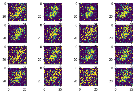
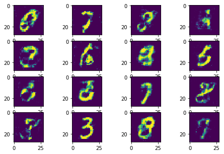In this improved version, the model collapse has been avoided as much as possible. The training process is much stable and much faster to converge.