Gaussian filtering

Control · 20 Feb 2019

This notebook introduces three common gaussian filters, Kalman filter, extended Kalman filter and unscented Kalman filter. Each filter has been implemented in Python and tested with a simple 3-order system. It highlights the feature of each filter and compares the performance between EKF and UKF. The thorough theory behind can be found at Wiki.

Note that the implementation of each filter isn’t polished for coding performance, since this blog focuses on the theory.

Linear system

3-order linear time invariant system

\[x_{k+1} = \begin{bmatrix} 1 & 0 & 1 \\ 0 & 1 & 1 \\ 0 & 0 & 0 \end{bmatrix}x_k + \begin{bmatrix} 0\\ 1\\ 1 \end{bmatrix}u + w\\ z_{k+1} = \begin{bmatrix} 1 & 0 & 0\\ 0 & 1 & 0\\ 0 & 0 & 1\\ \end{bmatrix}x_{k+1} + v\]

where process noise and measurement noise are \(w \sim \cal{N}(0, Q), v\sim \cal{N}(0,R)\).

A = np.array([[1, 0, 1], [0, 1, 1], [0,0,0]])
B = np.array([0,1,1]).reshape(-1,1)
C = np.eye(3)
# Check observability
obs_mat = np.concatenate([C, np.dot(C,A), np.dot(np.dot(C,A), A)], axis=0)
assert np.linalg.matrix_rank(obs_mat)==3
    
def state_update(x0,u):
    x = np.dot(A,x0) + np.dot(B,u)
    return x

def obs_update(x):
    z = np.dot(C,x)
    return z

def LTI(x0, u):
    x = state_update(x0,u)
    z = obs_update(x)
    return x,z

def run_linear(T):
    x0 = np.array([0,0,0]).reshape(-1,1)
    state_traj = np.zeros((3, T))
    obs_traj = np.zeros((3,T))
    Q = [[0.2,0,0], [0,0.1,0], [0,0,0.2]]
    R = [[10,0,0], [0,20,0], [0,0,18]]
    actions = []

    for i in range(T):
        w = np.random.multivariate_normal([0,0,0], Q).reshape(-1,1)
        v = np.random.multivariate_normal([0,0,0], R).reshape(-1,1)
        u = 20*np.random.rand()-10
        x,z = LTI(x0, u)

        x += w
        z += v
        state_traj[:, i:i+1] = x
        obs_traj[:, i:i+1] = z
        actions.append(u)

        x0 = x
    return state_traj, obs_traj, actions, Q, R

Nonlinear system

3-order nonlinear time invariant system

\[x_{k+1} = \begin{bmatrix} 15\sin{x_k^0}+u\\ x_k^0-10\cos{x_k^1}\\ x_k^0+x_k^2-u \end{bmatrix} + w\\ z_{k+1} = \begin{bmatrix} 1 & 0 & 0\\ 0 & 1 & 0\\ 0 & 0 & 1\\ \end{bmatrix}x_{k+1} + v\]

where process noise and measurement noise are \(w \sim \cal{N}(0, Q), v\sim \cal{N}(0,R)\).

def n_state_update(x0,u):
    x = np.zeros_like(x0)
    x[0] = 15*np.sin(x0[0])+u
    x[1] = x0[0] - 10*np.cos(x0[1])
    x[2] = x0[0] + x0[2]-u
    
    grad = np.zeros((3,3))
    grad[0,0] = 15*np.cos(x0[0])
    grad[1,0] = 1.0
    grad[1,1] = 10*np.sin(x0[1])
    grad[2,0] = 1.0
    grad[2,2] = 1.0
    
    return x,grad

def n_obs_update(x):
    C = np.eye(3)
    z = np.dot(C,x)
    
    grad = C
    return z, grad

def NLTI(x0, u):
    x,_ = n_state_update(x0,u)
    z,_ = n_obs_update(x)
    return x,z

def run_nonlinear(T):
    x0 = np.array([0.0,0.0,0.0]).reshape(-1,1)
    state_traj = np.zeros((3,T))
    obs_traj = np.zeros((3,T))
    Q = [[0.2,0,0], [0,0.1,0], [0,0,0.2]]
    mu_Q = [0.0,0.0,0.0]
    R = [[10,0,0], [0,20,0], [0,0,18]]
    mu_R = [0.0,0.0,0.0]
    actions = []

    for i in range(T):
        w = np.random.multivariate_normal([0,0,0], Q).reshape(-1,1)
        v = np.random.multivariate_normal([0,0,0], R).reshape(-1,1)
        u = 10*np.random.rand()-5
        x,z = NLTI(x0, u)

        x += w
        z += v
        state_traj[:,i:i+1] = x
        obs_traj[:,i:i+1] = z
        actions.append(u)

        x0 = x
    return state_traj, obs_traj, actions, Q, R, mu_Q, mu_R

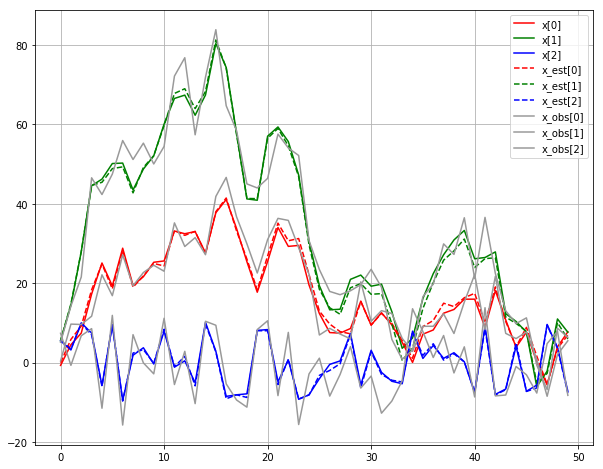
def plot_est(true, est, obs, plot_obs=False):
    plt.plot(true[0,:], 'r', label='x[0]')
    plt.plot(true[1,:], 'g', label='x[1]')
    plt.plot(true[2,:], 'b', label='x[2]')

    plt.plot(est[0,:], '--r', label='x_est[0]')
    plt.plot(est[1,:], '--g', label='x_est[1]')
    plt.plot(est[2,:], '--b', label='x_est[2]')
    if plot_obs:
        plt.plot(obs[0,:], '0.6', label='x_obs[0]')
        plt.plot(obs[1,:], '0.6', label='x_obs[1]')
        plt.plot(obs[2,:], '0.6', label='x_obs[2]')

Kalman filtering

Works well if following conditions are satisfied:

Linear system
Accurate modeling of state transition and measurement process
Good estimation of covariance at process noise and measurement noise

def kalman_filtering(u, x0_est, P0, z0, Q0, R0):
    # Prediction
    x1_0_est = state_update(x0_est, u)
    P1_0 = np.dot(np.dot(A,P0), A.transpose()) + Q0
    
    # Update
    residual = z0-obs_update(x1_0_est)
    S1 = np.dot(np.dot(C, P1_0), C.transpose()) + R0
    K1 = np.dot(np.dot(P1_0, C.transpose()), np.linalg.inv(S1))
    x1_1_est = x1_0_est+np.dot(K1, residual)
    P1_1 = np.dot((np.eye(A.shape[0])-np.dot(K1, C)), P1_0)
    
    return x1_1_est, P1_1

T = 50
state_traj, obs_traj, actions, Q, R = run_linear(T)

x0 = np.array([0,0,0]).reshape(-1,1)
P0 = np.zeros(3)

x_est_traj = np.zeros((3, T))
for i in range(T):
    x, P = kalman_filtering(actions[i], x0, P0, obs_traj[:, i:i+1].reshape(-1,1), np.asarray(Q), np.asarray(R))
    
    P0 = P
    x0 = x
    x_est_traj[:, i:i+1] = x

plt.figure(figsize=(10,8))
plot_est(state_traj, x_est_traj, obs_traj, True)
plt.legend()
plt.grid()

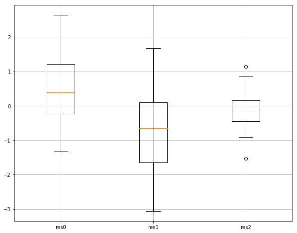
plt.figure(figsize=(10,8))
plt.boxplot(np.transpose(x_est_traj-state_traj), labels=['res0', 'res1', 'res2'])
plt.grid()
    

EKF

EKF is very similar to Kalman filter. The concept is the classic Kalman filter can be directly applied if the systme is differentiable. At each current state, if we can compute the jacobin of the system, the linearized system will be used in Kalman filter. The performance of EKF mainly depends on the accuracy and feasibility of linearization.

def extended_kalman_filtering(u, x0_est, P0, z0, Q0, R0):
    # Prediction
    x1_0_est, grad_state = n_state_update(x0_est, u)
    P1_0 = np.dot(np.dot(grad_state,P0), grad_state.transpose()) + Q0
    
    # Update
    z_est, grad_obs = n_obs_update(x1_0_est)
    residual = z0-z_est
    S1 = np.dot(np.dot(grad_obs, P1_0), grad_obs.transpose()) + R0
    K1 = np.dot(np.dot(P1_0, grad_obs.transpose()), np.linalg.inv(S1))
    x1_1_est = x1_0_est+np.dot(K1, residual)
    P1_1 = np.dot((np.eye(x0_est.shape[0])-np.dot(K1, grad_obs)), P1_0)
    
    return x1_1_est, P1_1


def run_ekf(x0, P0, actions, obs_traj, Q, R, T):
    x_est_traj = np.zeros((3,50))
    for i in range(50):
        x, P = extended_kalman_filtering(actions[i], x0, P0, obs_traj[:,i:i+1].reshape(-1,1), np.asarray(Q), np.asarray(R))

        P0 = P
        x0 = x
        x_est_traj[:,i:i+1] = x
    return x_est_traj



    

UKF

UKF samples \(2L+1\) sigma points around the mean, where \(L\) is the dimension sum of state and noise. Each point can be propagated through the nonlinear system. Thus, these sigma points can be used to form a new mean and covariance estimation.

def unscented_kf(u, x0_est, P0, z0, Q0, R0, mean_Q, mean_R, alpha, beta, gamma):
    # Prediction
    x_aug = np.concatenate([x0_est, mean_Q], axis=0)
    
    P_aug = np.block([[P0, np.zeros((3,3))],[np.zeros((3,3)), Q0]])
    
    
    dim_aug = x_aug.shape[0]
    
    sigma_points = [x_aug]
    lam = alpha**2*(dim_aug+gamma)-dim_aug
    term = cholesky((dim_aug+lam)*P_aug)
    term = np.transpose(term)
    for i in range(dim_aug):
        sigma_points.append(x_aug+term[:,i:i+1])
        sigma_points.append(x_aug-term[:,i:i+1])
    sigma_points_update=np.zeros((3, 2*dim_aug+1))
    for i in range(2*dim_aug+1):
        state,_ = n_state_update(sigma_points[i][:3,:],u)
        sigma_points_update[:,i:i+1] = (state+sigma_points[i][3:,:])
    
    x1_0_est = np.zeros_like(x0_est)
    for i in range(2*dim_aug+1):
        if i==0:
            w_s = lam/(lam+dim_aug)
            w_c = w_s + (1-alpha**2+beta)
        else:
            w_s = 1.0/(2*(dim_aug+lam))
            w_c = w_s
        x1_0_est += w_s*sigma_points_update[:,i:i+1]
        
    P1_0 = np.zeros_like(P0)
    for i in range(2*dim_aug+1):
        term = sigma_points_update[:,i:i+1]-x1_0_est
        P1_0 += w_c*np.outer(term,term)
    
        
    # Update
    x_aug = np.concatenate([x1_0_est, mean_R], axis=0)
    P_aug = np.block([[P1_0, np.zeros((3,3))], [np.zeros((3,3)), R0]])
    
    sigma_points = [x_aug]
    
    term = cholesky((dim_aug+lam)*P_aug)
    term = np.transpose(term)
    for i in range (dim_aug):
        sigma_points.append(x_aug+term[:,i:i+1])
        sigma_points.append(x_aug-term[:,i:i+1])
    
    assert len(sigma_points)==13
    sigma_points_update=[]
    for i in range(2*dim_aug+1):
        state,_ = n_obs_update(sigma_points[i][:3,:])
       
        sigma_points_update.append(state+sigma_points[i][3:,:])
    
    z_est = np.zeros_like(z0)
    for i in range(2*dim_aug+1):
        if i==0:
            w_s = lam/(lam+dim_aug)
            
        else:
            w_s = 1.0/(2*(dim_aug+lam))
           
        
        z_est += w_s*sigma_points_update[i]
    
    P_z_est = np.zeros_like(P0)
    P_s_z = np.zeros_like(P0)
    for i in range(2*dim_aug+1):
        if i==0:
            w_c = lam/(lam+dim_aug) + (1-alpha**2+beta)
        else:
            w_c = 1.0/(2*(dim_aug+lam))
        term = sigma_points_update[i]-z_est
        assert term.shape==(3,1)
        P_z_est += w_c*np.outer(term, term)
        
        P_s_z += w_c*np.dot(sigma_points[i][:3,:]-x1_0_est, np.transpose(sigma_points_update[i]-z_est))
    
    K = np.dot(P_s_z, np.linalg.inv(P_z_est))
    
    x1_1_est = x1_0_est+np.dot(K, z0-z_est)
    
    P1_1 =P1_0-np.dot(np.dot(K, P_z_est), np.transpose(K))
    
    return x1_1_est, P1_1
        

def run_ukf(x0, P0, actions, obs_traj, Q, R, mu_Q, mu_R, alpha, beta, gamma, T):

    x_est_traj = np.zeros((3,T))
    for i in range(T):
        x, P = unscented_kf(actions[i], x0, P0, obs_traj[:,i:i+1], np.asarray(Q), np.asarray(R), 
                            np.asarray(mu_Q).reshape(-1,1), np.asarray(mu_R).reshape(-1,1), alpha, beta, gamma)

        P0 = P
        x0 = x

        x_est_traj[:,i:i+1] = x
    return x_est_traj

Compare EKF & UKF

T = 50
state_traj, obs_traj, actions, Q, R, mu_Q, mu_R = run_nonlinear(T)

x0 = np.array([0.0,0.0,0.0]).reshape(-1,1)
P0 = np.diag([10.0, 10.0, 10.0])
alpha = 0.01
beta = 2.0
gamma = 0.0

ekf_est = run_ekf(x0, P0, actions, obs_traj, Q, R, T)
ukf_est = run_ukf(x0, P0, actions, obs_traj, Q, R, mu_Q, mu_R, alpha, beta, gamma, T)

plt.figure(figsize=(12,10))
plt.subplot(2,2,1)
plot_est(state_traj, ekf_est, obs_traj)
plt.legend()
plt.grid()
plt.title('EKF')

plt.subplot(2,2,3)
plt.boxplot(np.transpose(ekf_est-state_traj), labels=['res0', 'res1', 'res2'])
plt.grid()
plt.title('EKF')

plt.subplot(2,2,2)
plot_est(state_traj, ukf_est, obs_traj)
plt.legend()
plt.grid()
plt.title('UKF')

plt.subplot(2,2,4)
plt.boxplot(np.transpose(ukf_est-state_traj), labels=['res0', 'res1', 'res2'])
plt.grid()
plt.title('UKF')

Conclusion

For nonlinear system, UKF performs better than EKF, especially when the system is highly nonlinear. As we can see at the example above, UKF achieves better estimation at state \(x_3\) than EKF. For the estimation of the other two states, both have similar performance under the condition that EKF can compute the analytial result of jacobin.

However, the implementation of UKF is more complicated than EKF, which is just a linearization version of the classic Kalman filter. Although UKF doesn’t need information of jacobin, the computation of matrix square root is quite tricky.